Overview of VTAM
Aim
VTAM (Validation and Taxonomic Assignation of Metabarcoding Data) is a metabarcoding pipeline. The analyses start from high throughput sequencing (HTS) data of amplicons of one or several metabarcoding markers and produce an Amplicon Sequence Variant (ASV or variant) table of validated variants assigned to taxonomic groups.
Data curation (filtering) in VTAM addresses known technical artefacts: Sequencing and PCR errors, presence of highly spurious sequences, chimeras, internal or external contamination and dysfunctional PCRs.
One of the advantages of VTAM is the possibility to optimize filtering parameters for each dataset, based on control samples (Mock sample and negative control) to obtain results as close as possible to the expectations. The underlying idea is that if using these adjusted parameters for filtering provide clean controls, the real samples are also likely to be correctly filtered. Clean controls retaining all expected variants are the basis of comparability among different sequencing runs and studies. Therefore, the presence of negative control samples and at least one Mock sample is crucial.
VTAM can also deal with technical or biological replicates. These are not obligatory but strongly recommended to ensure repeatability.
Furthermore, it is also possible to analyse different primer pairs to amplify the same locus in order to increase the taxonomic coverage (One-Locus-Several-Primers (OLSP) strategy).
- Major steps:
Features of VTAM:
- Control artefacts to resolve ASVs instead of using clustering as a proxy for species
- Filtering steps use parameters derived from the dataset itself. Parameters are based on the content of negative control and mock samples; therefore, they are tailored for each sequencing run and dataset.
- Eliminate inter-sample contamination and Tag-jump and sequencing and PCR artefacts
- Include the analysis of replicates to assure repeatability
- Deal with One-Locus-Several-Primers (OLSP) data
- Assign taxa based on NCBI nt or custom database
Implementation
- VTAM is a command-line application running on linux, MacOS and Windows Subsystem for Linux (WSL ). It is implemented in Python3, using a conda environment to ensure repeatability and easy installation of VTAM and third party programmes:
- Wopmars (https://wopmars.readthedocs.io/en/latest/)
- ncbi-blast
- vsearch (Rognes et al., 2016)
- cutadapt (Martin, 2011)
- BLAST (Altschul et al., 1997)
- sqlite
The Wopmars workflow management system guarantees repeatability and avoids re-running steps when not necessary. Data is stored in a sqlite database that ensures traceability.
The pipeline composed of six scripts run as subcommands of vtam:
- vtam merge: Merges paired-end reads from FASTQ to FASTA files
- vtam sortreads reads: Trims and demultiplexes reads based on sequencing tags
- vtam optimize: Finds optimal parameters for filtering
- vtam filter: Creates ASVs, filters sequence artefacts and writes ASV tables
- vtam taxassign: Assigns ASVs to taxa
- vtam pool: Pools the final ASV tables of different overlapping markers into one
There are a few additional subcommands to help users:
- vtam random_seq Creates a random subset of sequences from fastafiles (recommended after the merge command)
- vtam make_known_occurrences to create known occurrence file automatically for the optimize step
- vtam taxonomy: Creates a taxonomic TSV file for the taxassign
- vtam example: Generates an example dataset for immediate use with VTAM
Although the pipeline can vary in function of the input data format and the experimental design, a typical pipeline is composed of the following steps in this order :
- vtam merge (optional)
- vtam random_seq (optional; useful if strong variation of the number of reads among replicates, or too many reads)
- vtam sortreads reads (optional)
- vtam filter (with default, low stringency filtering parameters)
- vtam taxassign (optional; useful, if the sequences of expected variants are NOT known in advance)
- vtam make_known_occurrences (optional; usefull if the sequences of expected variants are known in advance)
- vtam optimize
- vtam filter (with optimized parameters)
- vtam pool (if more than one markers or runs)
- vtam taxassign
The command vtam filter should be run twice. First, with default, low stringency filtering parameters. This produces an ASV table that is still likely to contain some occurrences which should be filtered out. Users should identify from this table clearly unexpected occurrences (variants present in negative controls, unexpected variants in mock samples, variants appearing in a sample of incompatible habitat) and expected occurrences in mock samples. This can be done either manually (for example if the sequences of expected varinats are not known in advance) or using the vtam make_know_occurrences command. Based on these occurrences, vtam optimize will suggest the most suitable parameters that keep all expected occurrences but eliminate most unexpected ones. Then, the command vtam filter should be run again, with the optimized parameters.
vtam taxassign has a double role: It will assign ASVs in an input TSV file to taxa, and complete the input TSV file with taxonomic information. The lineages of ASV are stored in a sqlite database to avoid re-running the assignment several times for the same sequence. Therefore running vtam taxassign the second or third time will be very quick and its main role will be to complete the input ASV table with taxonomic information.
If using several overlapping markers vtam pool can be run to pool the ASV tables of the different markers. In this step variants identical in their overlapping regions are pooled together. vtam pool can also be used to simply produce one single ASV table from several different runs.
Input data structure
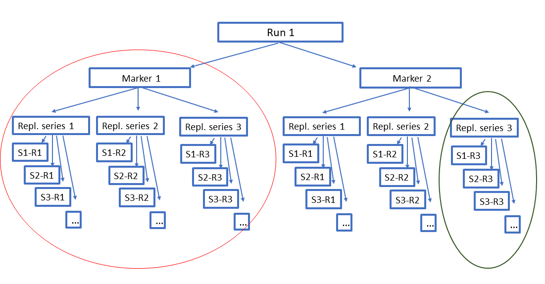
Figure 1. Input data structure.
The filtering in VTAM is done separately for each run-marker combination. Different runs can be stored in the same database, allowing to pool all the results into the same ASV table.
In case of more than one strongly overlapping markers, the results of the same run(s) for different markers can also be pooled. Variants identical in their overlapping regions are pooled and presented in the same line of the ASV table.
Replicates are not mandatory, but very strongly recommended to assure repeatability of the results.
- Samples belong to 3 categories:
- Mock samples have a known DNA composition. They correspond to an artificial mix of DNA from known organisms.
- Negative controls should not contain any DNA.
- Real samples have an unknown composition. The aim is to determine their composition.
Negative controls and at least one mock sample are required for optimising the filtering parameters.
The mock sample should ideally contain a mix of species covering the taxonomic range of interest and reflect the expected diversity of real samples. It is not essential to have their barcode sequenced in advance if they come from a well-represented taxonomic group in the reference database. In that case, their sequences can be generally easily identified after running the filtering steps and taxonomic assignations with default parameters. However, if there are several species from taxonomic groups weakly represented in the reference database, it is better to barcode the species before adding them to the mock sample. It is preferable to avoid using tissue that can contain non-target DNA (e.g. digestive tract).
Mock samples can contain species that are impossible to find in the real samples (e.g. a butterfly in deep ocean samples). These species are valuable to detect tag jump or inter-sample contaminations in real samples, and thus help to find optimal parameter values of some of the filtering steps. Alternatively, real samples coming from markedly different habitats can also help in the same way.